Plot low-dimensional embedding

This example shows how to plot a low-dimensional embedding of the rhythmic patterns.

This is based on the rhythmic patterns analysis proposed in [CIM2014].

# Code source: Martín Rocamora
# License: MIT

Imports

• matplotlib for visualization
• Axes3D from mpl_toolkits.mplot3d for 3D plots

from __future__ import print_function
import matplotlib.pyplot as plt
from mpl_toolkits.mplot3d import Axes3D
import carat

We compute the feature map of rhythmic patterns and we learn a manifold in a low–dimensional space. The patterns are they shown in the low–dimensional space before and after being grouped into clusters.

First, we’ll load one of the audio files included in carat.

audio_path = carat.util.example_audio_file(num_file=1)

y, sr = carat.audio.load(audio_path)

Next, we’ll load the annotations provided for the example audio file.

annotations_path = carat.util.example_beats_file(num_file=1)

beats, beat_labs = carat.annotations.load_beats(annotations_path)
downbeats, downbeat_labs = carat.annotations.load_downbeats(annotations_path)

Then, we’ll compute the accentuation feature.

Note: This example is tailored towards the rhythmic patterns of the lowest sounding of the three drum types taking part in the recording, so the analysis focuses on the low frequencies (20 to 200 Hz).

acce, times, _ = carat.features.accentuation_feature(y, sr, minfreq=20, maxfreq=200)

Next, we’ll compute the feature map.

n_beats = int(round(beats.size/downbeats.size))
n_tatums = 4

map_acce, _, _, _ = carat.features.feature_map(acce, times, beats, downbeats, n_beats=n_beats,
                                               n_tatums=n_tatums)

Then, we’ll group rhythmic patterns into clusters. This is done using the classical K-means method with Euclidean distance (but other clustering methods and distance measures can be used too).

Note: The number of clusters n_clusters has to be specified as an input parameter.

n_clusters = 4

cluster_labs, centroids, _ = carat.clustering.rhythmic_patterns(map_acce, n_clusters=n_clusters)

Next, we compute a low-dimensional embedding of the rhythmic pattern. This is mainly done for visualization purposes. This representation can be useful to select the number of clusters, or to spot outliers. There are several approaches for dimensionality reduction among which isometric mapping, Isomap, was selected (other embedding methods can be also applied). Isomap is preferred since it is capable of keeping the levels of similarity among the original patterns after being mapped to the lower dimensional space. Besides, it allows the projection of new patterns onto the low-dimensional space.

Note 1: You have to provide the number of dimensions to map on. Although any number of dimensions can be used to compute the embedding, only 2- and 3-dimensions plots are available (for obvious reasons).

Note 2: 3D plots need Axes3D from mpl_toolkits.mplot3d

n_dims = 3
map_emb = carat.clustering.manifold_learning(map_acce, method='isomap', n_components=n_dims)

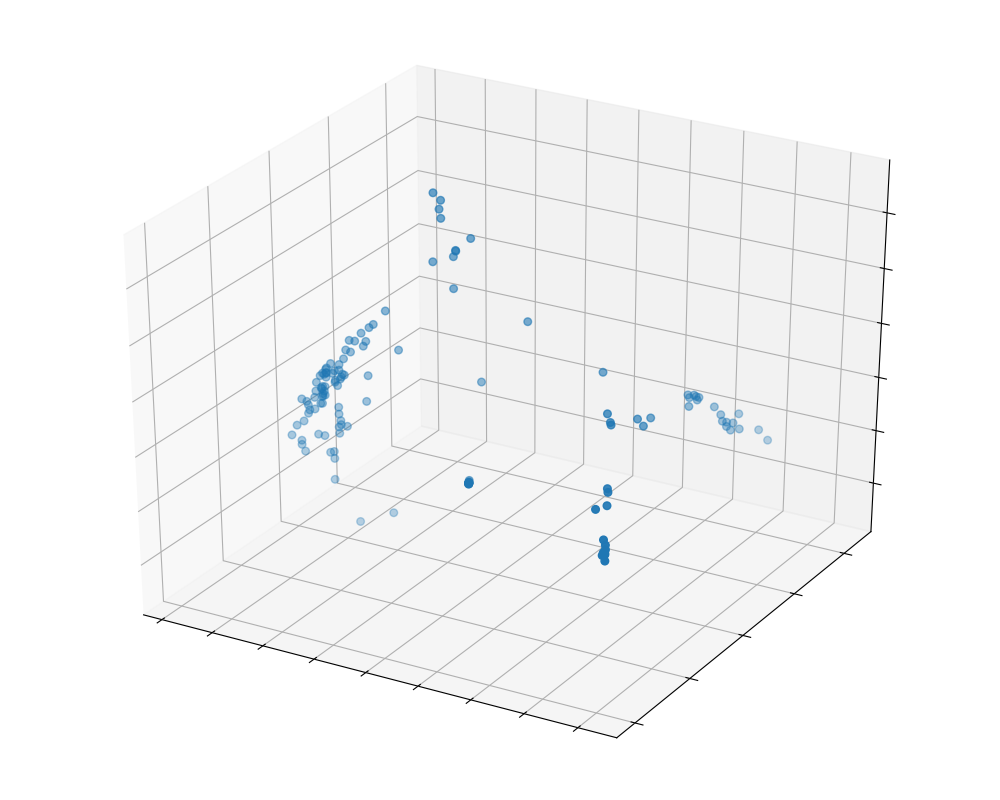
Finally we plot the low-dimensional embedding of the rhythmic patterns and the clusters obtained.

fig1 = plt.figure(figsize=(10, 8))
ax1 = fig1.add_subplot(111, projection='3d')
carat.display.embedding_plot(map_emb, ax=ax1, clusters=cluster_labs, s=30)
plt.tight_layout()

fig2 = plt.figure(figsize=(10, 8))
ax2 = fig2.add_subplot(111, projection='3d')
carat.display.embedding_plot(map_emb, ax=ax2, s=30)
plt.tight_layout()

plt.show()

• 
•