Plot feature map

This example shows how to compute a feature map from de audio waveform.

This type of feature map for rhythmic patterns analysis was first proposed in [CIM2014].

[CIM2014]

Tools for detection and classification of piano drum patterns from candombe recordings. Rocamora, Jure, Biscainho. 9th Conference on Interdisciplinary Musicology (CIM), Berlin, Germany. 2014.

# Code source: Martín Rocamora
# License: MIT

Imports

• matplotlib for visualization

from __future__ import print_function
import matplotlib.pyplot as plt
import carat

The accentuation feature is organized into a feature map. First, the feature signal is time-quantized to the rhythm metric structure by considering a grid of tatum pulses equally distributed within the annotated beats. The corresponding feature value is taken as the maximum within window centered at the frame closest to each tatum instant. This yields feature vectors whose coordinates correspond to the tatum pulses of the rhythm cycle (or bar). Finally, a feature map of the cycle-length rhythmic patterns of the audio file is obtained by building a matrix whose columns are consecutive feature vectors.

First, we’ll load one of the audio files included in carat.

audio_path = carat.util.example_audio_file(num_file=1)

y, sr = carat.audio.load(audio_path)

Next, we’ll load the annotations provided for the example audio file.

annotations_path = carat.util.example_beats_file(num_file=1)

beats, beat_labs = carat.annotations.load_beats(annotations_path)
downbeats, downbeat_labs = carat.annotations.load_downbeats(annotations_path)

Then, we’ll compute the accentuation feature.

Note: This example is tailored towards the rhythmic patterns of the lowest sounding of the three drum types taking part in the recording, so the analysis focuses on the low frequencies (20 to 200 Hz).

acce, times, _ = carat.features.accentuation_feature(y, sr, minfreq=20, maxfreq=200)

Next, we’ll compute the feature map. Note that we have to provide the beats, the downbeats, which were loaded from the annotations. Besides, the number of beats per bar and the number of of tatums (subdivisions) per beat has to be provided.

n_beats = int(round(beats.size/downbeats.size))
n_tatums = 4

map_acce, _, _, _ = carat.features.feature_map(acce, times, beats, downbeats, n_beats=n_beats,
                                               n_tatums=n_tatums)

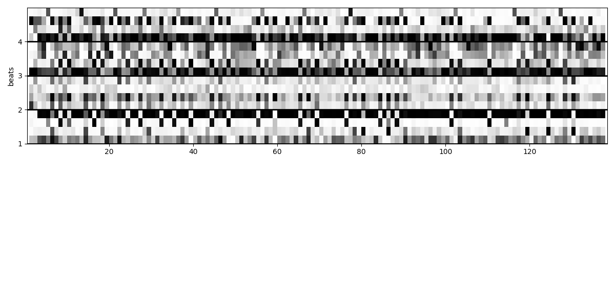
Finally we plot the feature map for the low frequencies of the audio file.

Note: This feature map representation enables the inspection of the patterns evolution over time, as well as their similarities and differences, in a very informative way. Note that if a certain tatum pulse is articulated for several consecutive bars, it will be shown as a dark horizontal line in the map. Conversely, changes in repetitive patterns are readily distinguishable as variations in the distribution of feature values.

plt.figure(figsize=(12, 6))
ax1 = plt.subplot(211)
carat.display.map_show(map_acce, ax=ax1, n_tatums=n_tatums)
plt.tight_layout()

plt.show()